Deploying Abaqus on Rescale to Stress Test Compliant Mechanisms
Overview
A compliant mechanism is a mechanism that gains at least some of its mobility from the deflection of flexible members rather than from movable joints only. By using flexible joints, we can decrease the part count, simplify production, decrease price and increase portability of the mechanism.

This two degree-of-freedom pointer device uses compliant mechanism technology to obtain its motion. It was developed by the BYU Compliant Mechanisms Research group (compliantmechanisms.byu.edu), under a grant from NASA.
Traditional pointing mechanisms like gimbals have multiple moving and pinching parts which can cause damage to fuel pipes or wires connected to the thruster or antenna. On the other hand, the compliant mechanism is a single unit which can be 3d-printed. It also has no pinch zones.

In this tutorial, I will use an Abaqus CAE Interactive workflow in Rescale to stress test a modelA numerical, symbolic, or logical representation of a system... More of this compliant mechanism. Since many of the flexible members undergo large deflections, linearized beam equations are no longer valid. Nonlinear equations must be used that account for the geometric nonlinearities caused by large deflections. So we will use HPCThe use of parallel processing for running advanced applicat... More to simplify and speedup this intensive workflow.
I will first walkthrough setting up the workstationA workstation is a powerful computer system designed for pro... More and then perform the analysis. The file attached in this tutorial is the STEP file of the model, this was generated manually on Onshape following the outline of the original STL file. The new file is better suited to FEA modelingModeling is the creation of a mathematical or conceptual rep... More as it is made up of simpler parts and describes the model better than the original STL file, which uses point based modeling for which Abaqus generates too many faces.
Video Tutorial
Configuring Your Workstation
- First, we navigate to the workstations tab and select New Workstation. We will then be directed to upload our input files. The file pointer_smoothed.step is uploaded here and you should see it in the box below.


- Next, we navigate to software selection and select Abaqus CAE Interactive Workflow as our software and use the on demand license.


- Now we navigate to the the hardware selection screen. Here I choose the Citrine coretypePre-configured and optimized architectures for different HPC... More from the coretype explorer since Citrine comes with better graphics capabilities which helps in interacting with the model in Abaqus. I select 16 cores with a wall-time of 10 hours and submit the workstation.


- Resources for the workstation will start provisioning and when the workstation is ready, a connect button will appear through which we can remotely connect with our desktop.
On the Workstation
- After the workstation has launched we can open the Abaqus software and import the pointer mechanism as a part. All uploaded files will be in work > shared directory.


- After Abaqus reads the file we can begin our analysis. The workflow that I will follow can be below, in the dropdown menu module we start from the top and work our way down in the order Property > Assembly > Step > Load > Mesh > Job. I will describe what to do in each of these sections to get the final results.

- In the Property module, we describe the materials and sections used in our simulationSimulation is experimentation, testing scenarios, and making... More. There are three things to do in this module, the buttons are highlighted in the screenshot and they must be clicked from top to bottom. Clicking the first one would prompt us to describe a material.
- Choose Mechanical > Elastic and your material would require Young’s Modulus and Poisson’s Ratio. The value for PLA of these measurements are 4e9 for Young’s Modulus and 0.337 for the Poisson’s Ratio. Input these to create the PLA material.
- Next button would prompt us to create a section, make sure the section is solid and homogenous.
- The third button would prompt us to assign the section to the part. So we click the part which selects the entirety of it and click done to assign PLA to our mechanism.


- In the Assembly module, all we have to do is click the first button and load out part into assembly.

- In the Step module, we describe the type of analysis we will do. Click the first button and select Static,General as the type of analysis. In the next prompt TURN NON-LINEAR GEOMETRY ON.

- In the Load module we describe the boundary conditions and forces we want to place on our mechanism. We click the second button to set the boundary condition of where the mechanism would be attached to the rest of the body. Since the part attached doesn’t move, we select a displacement boundary condition and set all changes in displacement to zero on the highlighted part.


- We do another boundary condition to describe a displacement of one of the force input points. This is the main force that I intend to analyze, I opt for a boundary condition instead of a pressure or force since we need to worry less about the exact calculations of force and the size of the area it is applied to. Follow the same steps as the previous one but set the change in z-coordinate to be -150e-06. The face it is applied to is shown in the picture below.

- The next module is Mesh. Here first we select Part instead of Assembly at the top. Then we do the steps in the order listed in the picture below; Seed Part > Assign Mesh Controls > Mesh Part.
- In the first step, we select a seed size. A size that worked for me was 0.000018 (Note: The size in the screenshot is 10x bigger than what it is supposed to be).
- Then we assign Tet mesh controls to the whole part.
- Finally we mesh the part, this can be time consuming.


- With everything set up, we can submit the job and take advantage of the parallelization. Navigate to the Jobs module and create a new job with parallelization set to 16 corean individual processing unit within a multicore processor o... More. Submit this job and wait for the results.


Results
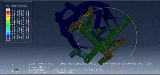
After the job has finished, we can move on to the visualizationVisualization is the representation of complex scientific or... More module and plot the results of our analysis. The forces applied to the compliant mechanism in this example should rotate it to point in a different direction, and that is what we see when we plot the displacement in the animation below. We can also analyze the amount of von Mises stress that each part experiences, and we can see the flexible members undergo stress as was expected, specifically 75% of the yield criterion was the average.