
ANSYS Fluent Batch Tutorials
This tutorial will introduce you to submitting ANSYS jobs in batch to the Rescale platform. We will create an input file from the respective ANSYS software, start a Rescale job, submit, and transfer the results back to ANSYS.
Pre-processing activities (e.g. geometry, mesh/model) are already completed and all solverA solver is a numerical algorithm or a software tool that so... More and setup settings are already determined as well. Unlike job submission through RSM, you do not need to launch Rescale Desktops. You can use your own ANSYS software and license or reach out to us and purchase some Elastic License Units (ELUs).
In this section, we will solve an ANSYS Fluent job in batch. To obtain the files needed to follow this tutorial, click on the “Job Setup” link below and clone the job hosting the file. Next, click “Save” on the job to have a copy of the files in your Rescale cloud files.
Import Job Setup Get Job Results
The input files are:
tjunction_plot.cas.gz – Compressed Case File
run_plot.jou – Journal File
Creating Case and Journal files
In this section, we will solve an ANSYS Fluent job in batch. To obtain the files needed to follow this tutorial, click on the “Job Setup” link below and clone the job hosting the file. Next, click “Save” on the job to have a copy of the files in your Rescale cloud files.
The input files are:
tjunction_plot.cas.gz – Compressed Case File
run_plot.jou – Journal File
Creating Case and Journal files
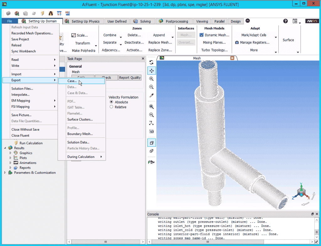
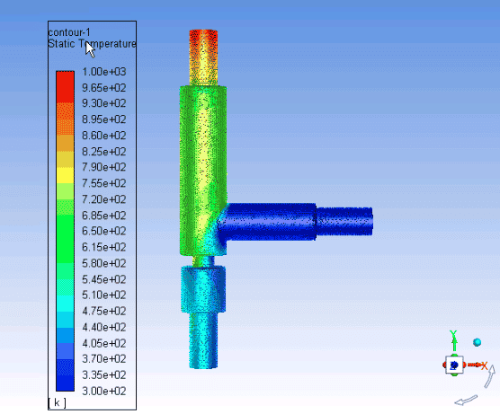
The tutorial example is a T-junction of two fluids at different temperatures using ANSYS Fluent version 18. The case file tjunction_plot.cas.gz is already available to you. The steps involved to create a case file are:
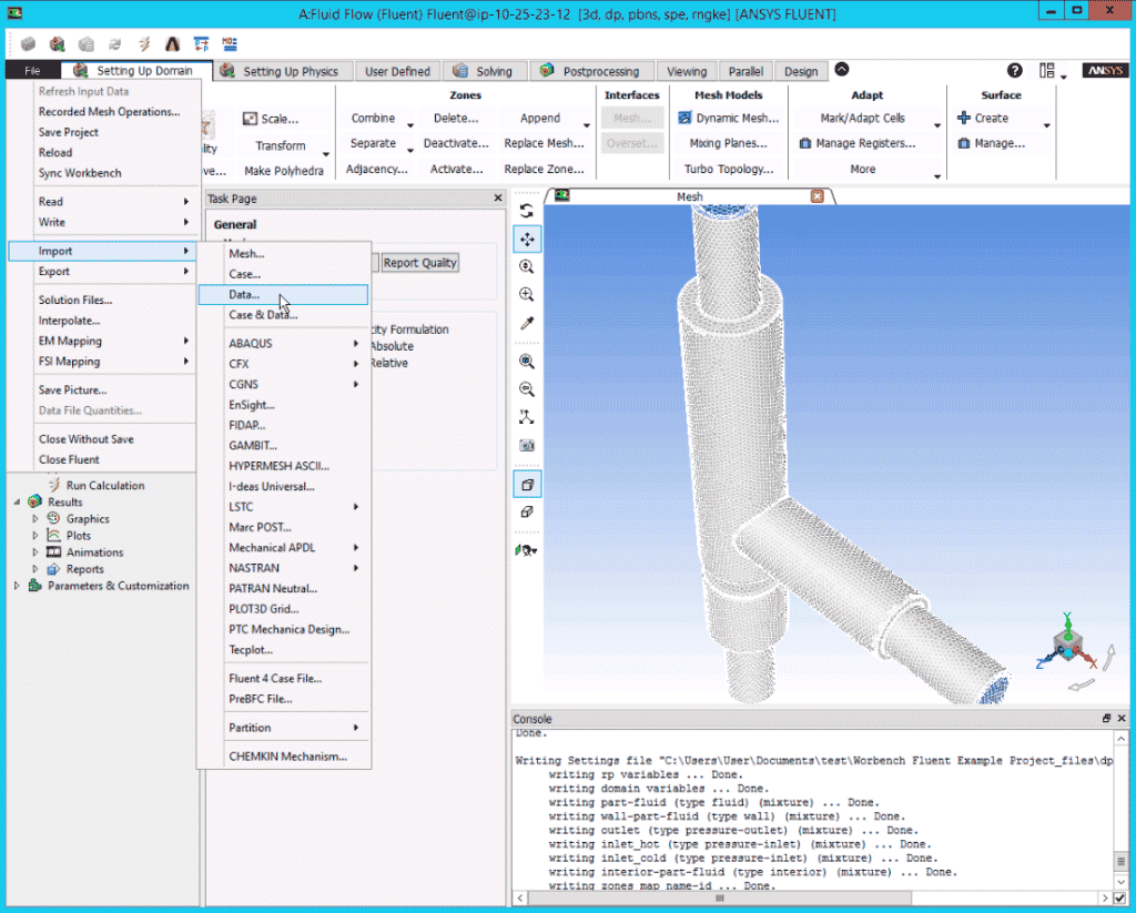
- On Fluent, go to the File tab, then select Export > Case…, and this will open a window browser
- Name the file with a .cas or .cas.gz extension and select the location where this file will be exported to.
This file contains all pre-processing settings, and solver and physics setup that have been configured in the GUI, as per your standard workflow.
You will also need a journal file which contains all the necessary commands that you would like to execute using Fluent during a batch run. The journal file run_plot.jou is already available to you. The steps involved to create a journal file are:
- On a Windows Explorer window, right mouse click > New > Text Document (or similar for other OS).
- Give the file a name, with extension .jou. Accept the change to file extension.
- Double-click the file to open it and enter the journal commands, then save the file.
The journal file will look like this:
/file/set-batch-options no yes yes no
/file/read-case tjunction_plot.cas
/solve/initialize/initialize/
/solve/iterate 500
/file/write-case-data tjunction_plot%i.cas.gz
/exit yes
The journal file shown above reads the case file, sets the batch options, initializes, runs the calculation for 500 iterations, and finally writes a case and a data file when the solution has converged to a prescribed limit.
This file is written using the ANSYS Fluent Text User Interface (TUI). For more information about using specific text interface commands, please refer to ANSYS Online Documentation here.
Rescale Job Setup
After obtaining the necessary ANSYS Fluent files, we will now submit a Basic job on Rescale. For more information on launching a basic job, please refer to the tutorial here.
Setup: Input File(s)
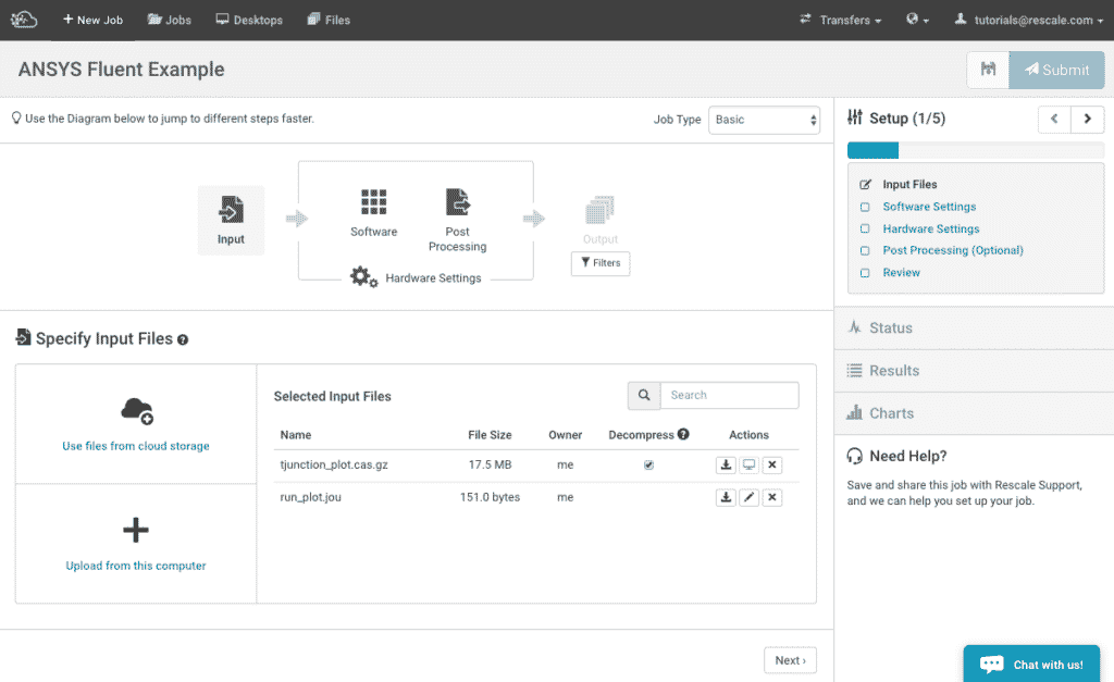
- Go onto the Rescale platform, click on + New Job on the top left. Name your job and make sure the Job Type is set to Basic.
- Next upload the journal and case files as input files.
Setup: Software Settings
Click Next to move onto the Software Settings section of the setup.
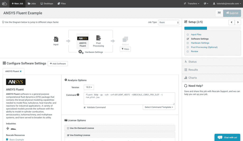
- You can scroll down or use the search bar to select ANSYS Fluent. The Analysis Options will display and select version 18.0.
- In the command window, you will need to specify the journal file name under the angle bracket <journal filename>. We would also like to see the solution residual. To do this, we command to keep the graphics windows using the -gu option.
- Next under LicensingLicensing is a legal tool granting users the rights to use, ... More Options, select Use Existing License and enter your ANSYS servera server is a computer program that provides services to oth... More connection port numbers under License and ANSYS License InterconnectTthe cabling and switches used by compute nodes to communica... More respectively.
For this tutorial, the software settings page will look as shown below.
Setup: Hardware Settings
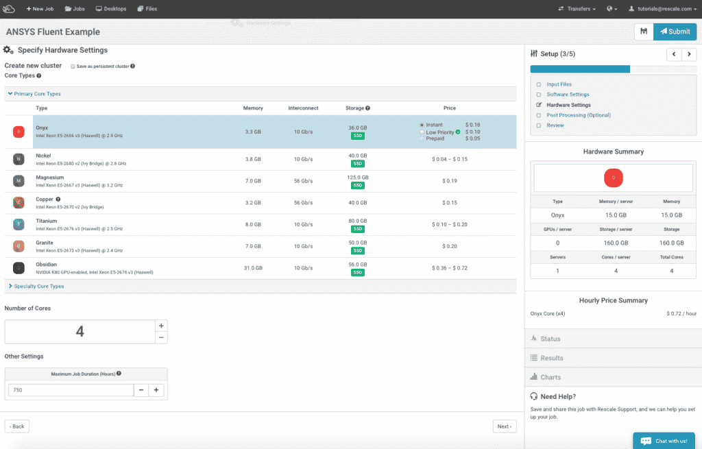
The next step is to select the desired hardware for the job. Click on the Hardware Settings icon.
- Select your desired corean individual processing unit within a multicore processor o... More type and the numbers of cores that you want to use for this job. For this tutorial, select Emerald and 4 cores.
Your Hardware Settings screen should look like this:
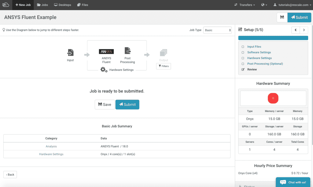
Setup: Review
There are no post-processing settings in this tutorial. Click on the Review icon. Check that the setup is correct by reviewing the Basic Job Summary table. It should look like this:
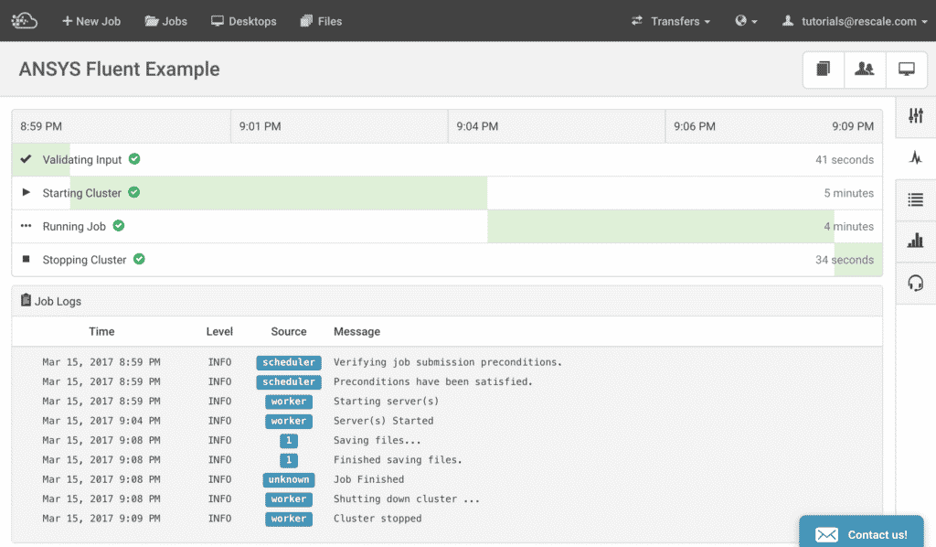
Job Submission and Monitor
Once you have reviewed your setup, you are ready to submit your job. Click Submit and you will move on from the Setup page to the Status page in the Rescale platform. Here, you will be able to monitor the job progress in a Gantt chart like format, see a date and time stamped log and live-tail the status and output of your job using the Live-tail window. A guide on “Monitoring Status” on Rescale is found here.
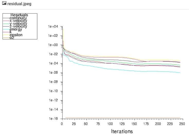
In this example, we have configured the simulationSimulation is experimentation, testing scenarios, and making... More to output a residual plot at every iteration, which will show up under the Live Tailingalso referred to as real-time log monitoring or live log str... More window as a residual.jpeg file. You can open this graph at any time to monitor the progress of the solution’s convergence.
Viewing Results
Once the job is completed, you can either view the results on your local workstationA workstation is a powerful computer system designed for pro... More or on a Rescale Desktop. Both methods are presented below:
On your Local Workstation
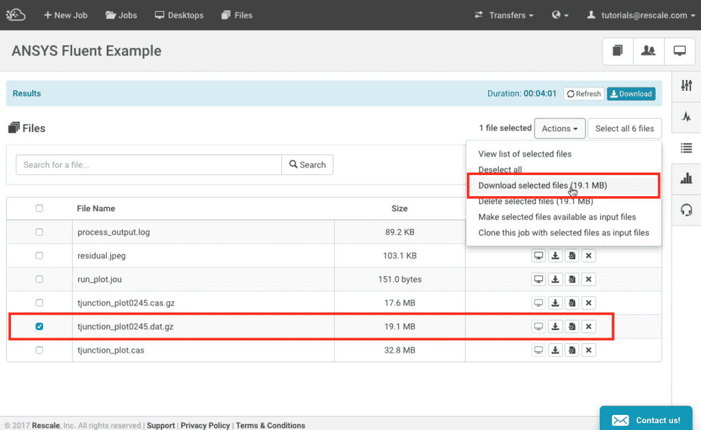
Once the job is completed, you can select the file(s) that you wish to download.
Note: If you have large output files, it is recommended that windows users use Rescale Transfer Manager (RTM) to download files faster onto your on-premises workstation. More information about RTM can be found here. Linux or Mac user can use Rescale CLI to download larger output files.
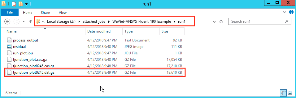
- Go to the results page of the completed job, find and select the
tjunction_plot0245.dat.gz - Go to Actions and click on Download selected files, give it a few seconds for it download to your computer
- Launch Fluent . Go to File tab, then select Import > Data… , to load the solution data file
On a Rescale Desktop
Once the job is completed, follow these steps to view results on a Rescale Desktop:
Set up a Desktop Session:
- Under 1.Choose Configuration dropdown, select the hardware for your Desktop Session
- Under 2.Add Software dropdown, select ANSYS Fluids Desktop
- Under 3.Jobs dropdown, search for the job you wish to add by typing the name and/or browsing through the list. Click Add to add a job to the Desktop
- Once the Desktop session is started, launch Fluent
- On Fluent, go to the File tab, then select Import > Data… . Navigate to the mapped directories. it is common to map to the Z: drive, but the attached job could be in the X: or Y: drives as well depending on your setup. Click on
tjunction_plot0245.dat.gzfile to load the solution data file and click Open
At this point, you can proceed to your post-processing activities as you would normally do after solving an Ansys Fluent simulation interactively.
ANSYS Fluent also has the capability of allowing users to modify or extend the behavior of the physics and solver setup. User defined functions (UDF) can be used to perform actions such as impose boundary conditions, physical and chemical processes, heat transfer and phase changes.
In this section we present instructions using Fluent User Defined Functions (UDF) in batch mode on the Rescale platform.
This guide will assume that you already have developed a UDF ready for compilation in a Fluent job. For assistance on creating or debugging UDFs please contact ANSYS Support directly. Here is a guide by ANSYS on using UDFs in Fluent.
Compilation of UDFs in Batch
To utilize a UDF during a batch run, the UDF source code must first be compiled and accessible by Fluent. We will demonstrate a workflow that compiles the UDF at runtime before the main solution solve or iteration process. We will accomplish this by adding commands to an existing example journal file. Depending on your workflow and the size of the compilation libraries, it is possible to have these UDF libraries pre-compiled and included as input files to your batch job. But generally UDFs are straightforward codes, so runtime compilation is a short operation and avoids any platform inconsistencies.
Example Journal File
The following is an example of a journal file that compiles a user-created custom_UDF.c file in current directory (with the journal file) and loads the resulting UDF libraries. The UDF is compiled with the default library name libudf and creates a correspondingly named directory structure with the shared libraries.
Here, the compilation and load commands (shown in bold) are sequential and take place before the solution initialization. But you can perform these operations anywhere they fit into your workflow.
/file/set-batch-options no yes yes no
/file/read-case example.cas
/define/user-defined/compiled-functions compile libudf yes custom_UDF.c ""

/define/user-defined/compiled-functions load libudf
/solve/initialize/initialize
/solve/iterate 1000
/parallel/timer/usage
/file/write-case-data example-%i.cas
/exit yes
There are two specific syntax things to note here. The first, is that after the UDF source code file name, there are two double quotes "" present. The second is the blank line after the compile command. This ensures that the compile function does not attempt to treat following lines as additional file names to include in the compile. The blank line is necessary after the compilation command but does not need to precede or follow the load command.
Making an Explicit UDF Call
Occasionally you will have to call a UDF function before or after a solution process to set up a boundary condition or perform some sort of post-processing step. You can call that UDF function explicitly in your journal file with an execute-on-demand call where appropriate:
/define/user-defined/execute-on-demand "FunctionName::libudf"
Running on Multiple Nodes
Another thing to note is that due to the nature of UDF function calls, all nodes need access to the compiled UDF libraries. By default, ANSYS Fluent jobs are set to run in the ~/work directory which is local to the head nodeIn traditional computing, a node is an object on a network. ... More. Depending on the behavior of the function, the worker node processes may need to access a common file or library. In this case, the job should be run out of the NFS mounted directory, ~/work/shared. So simply prepend move and change directory commands on the “Software Settings” page before you launch Fluent (not in the journal file):
mv * shared
cd shared
fluent 3ddp -gu -ssh -cnf=$FLUENT_HOSTS -t$RESCALE_CORES_PER_SLOT -i example.jou
So again, if you are running on multiple cores on a single node, this step is unnecessary since the local file system can be accessed by all the cores on that node.