ANSYS Fluent DOE Tutorial
In this tutorial, we show how to setup Design of Experiments (DOE)DOE stands for "Design of Experiments." It is a statistical ... More with variable design parameters for ANSYS Fluent simulations.
We will use a T-Junction mixing problem with cold and hot fluid inlets. At the T-Junction both fluids mix and result in a outlet temperature which is a design objective for this example. We will simulate to perform a parametric sweep of the different inlet temperatures using DOE job type option available on Rescale.
The job files for this tutorial can be accessed by clicking the Import Job Setup button below:
On the Rescale Platform
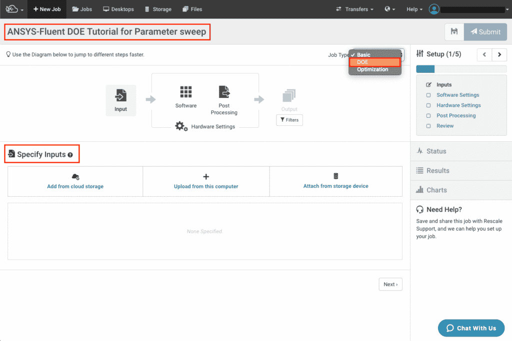
- Start by clicking +New Job
- Name the job appropriately
- Change the Job type to DOE as shown in the screen shot below
- You can see the platform configuration layout change to DOE setup
- Add input files using the Specify Inputs window
Further, use Add from Cloud Storagea simple and scalable way to store, access, and share data o... More or Upload from this computer options to upload the Fluent case modelA numerical, symbolic, or logical representation of a system... More, as shown below
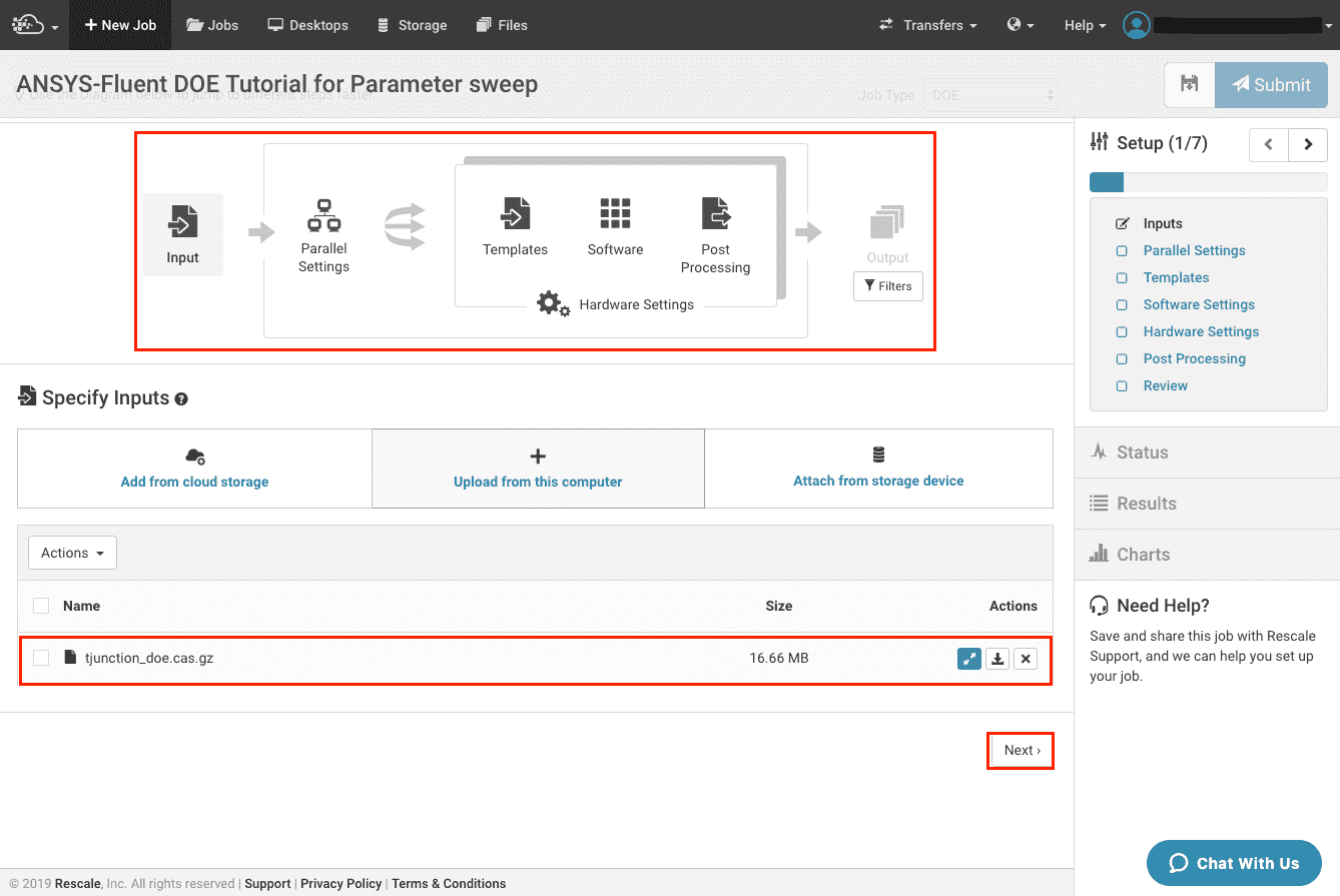
Click on Next button to go to Parallel Settings Page
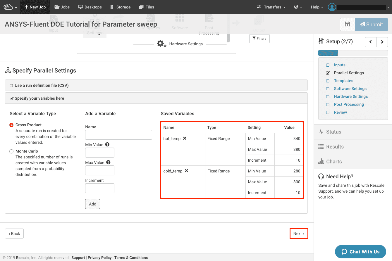
On the Parallel Settings page, we will specify the range of parameters for DOE simulation setup.
We can set the parameters:
- By specifying a
.csvfile using the option Use a run definition file - By manually entering the parameters using Specify your variables here as shown in the image below
Here, we can use Cross Product or Monte Carlo based sweep of the parameters.
- Cross Product option would generate all the combinations of the parameters to run the simulations
- Monte Carlo option would generate parameters based on the probability distribution specified
In this tutorial, we will use Cross Product option.
- Enter the variable
Name,Max Value,Min Valueand theIncrementto add it as a variable parameter as shown below.
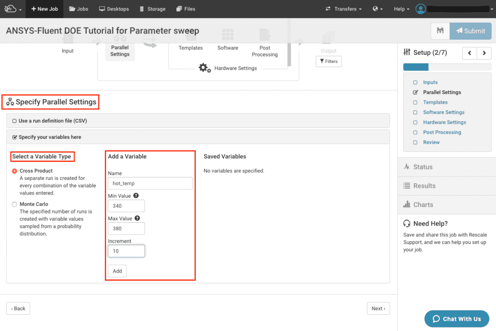
You can add as many variables for DOE simulations to be designed. Here, we have used two parameter variables cold_temp and hot_temp for this DOE (See below):
Once you have set all the variable parameters for the DOE simulation, move to the Templates page.
Here we will upload the template that will be used to create multiple .jou journal files for individual child runs.
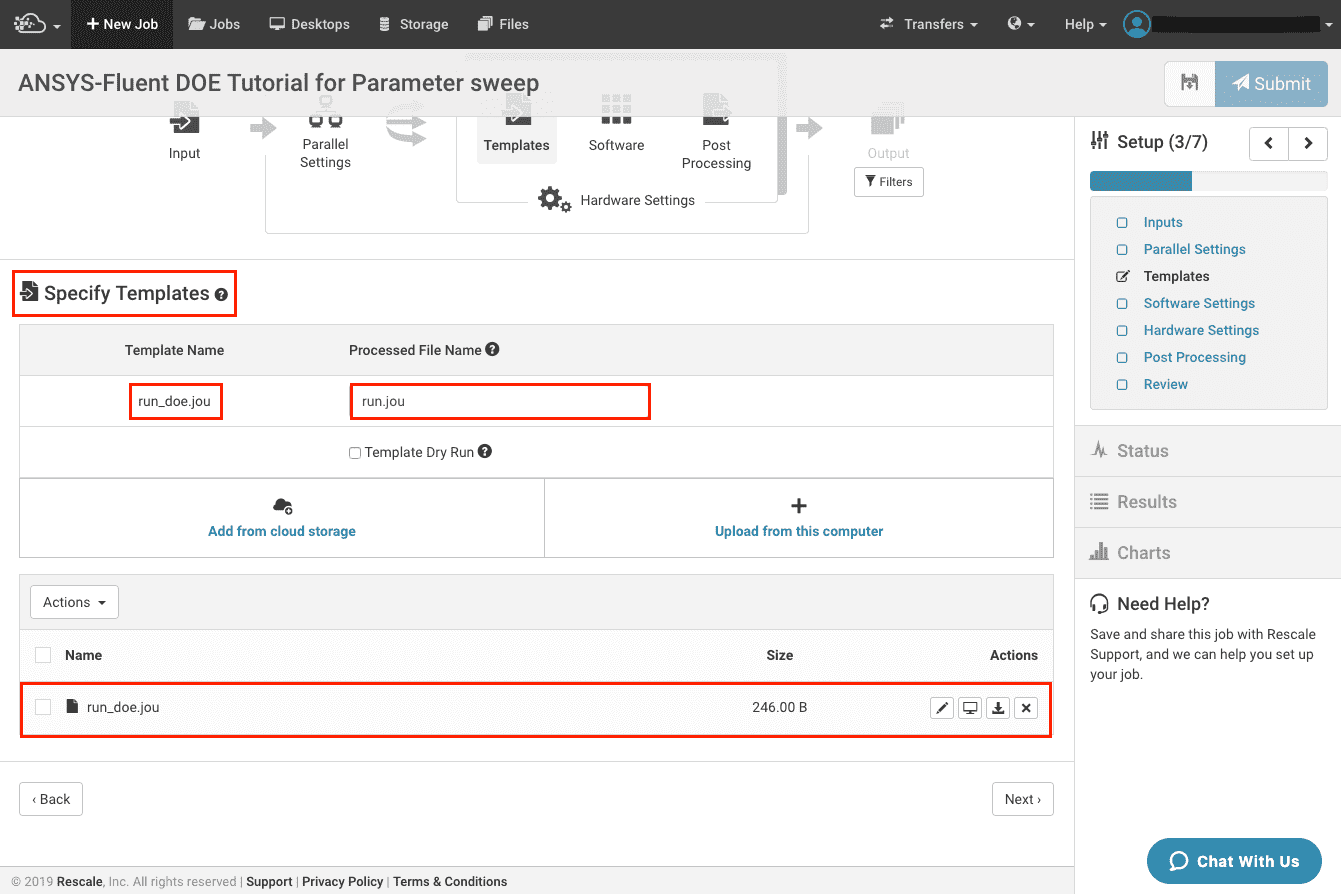
The run_doe.jou template file for this simulation is as follows:
/file/read-case tjunction_doe.cas/file/set-batch-options no yes yes no/define/boundary-conditions/vi inlet_cold ,,,,,,,, no , ${cold_temp} ,,,,,/define/boundary-conditions/vi inlet_hot ,,,,,,,, no , ${hot_temp} ,,,,,/solve/iterate 500/file/write-case-data tjunction_doe%i.cas.gz/exit yes
You can create this journal file from the GUI commands that are recorded as Scheme code lines in journal files. FLUENT creates a journal file by recording everything you type on the command line or enter through the GUI. You can also create journal files manually with a text editor. Once you create a simulation specific journal file you can use Rescale DOE option and create a template file similar to the one above to perform Fluent simulations with all the parameters.
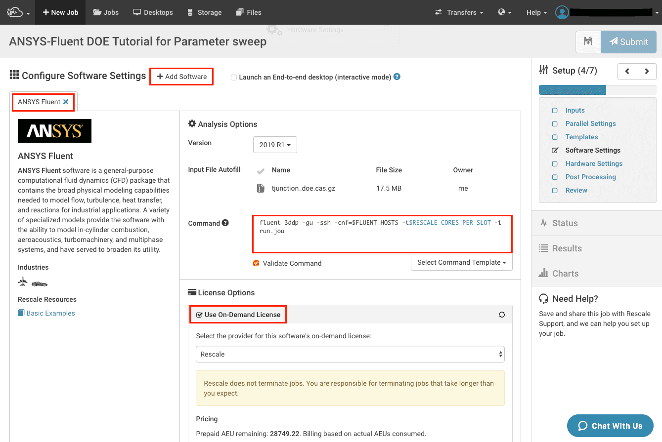
Click Next to move to Software Settings
After clicking +Add Software button, search with keywords fluent and select the ANSYS Fluent software from the menu. This would add the software and populate the relevant commands, versions required to run a Fluent simulation.
- In the command window at the end of the command add the name of the journal file. In this tutorial, the journal file name is
run.jou(see below). - Based on your preference select the License Options
- Select Use On-Demand License for purchasing license
- Select Use Existing License if this option is configured for your account
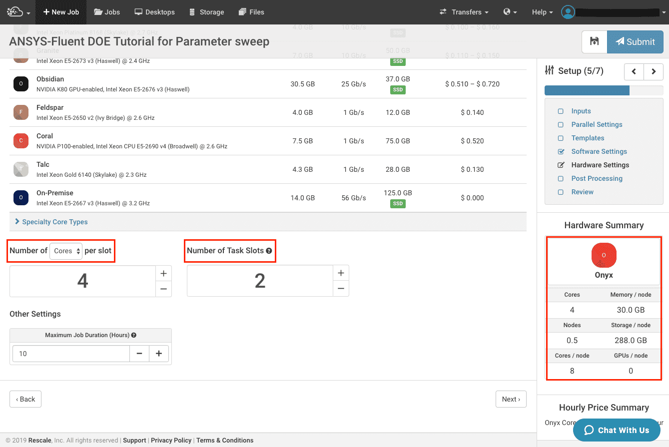
In this tutorial we will choose:
- Corean individual processing unit within a multicore processor o... More Type: Emerald with on-demand option
- Number of Cores per slot: 4
- Number of Task Slots: 2
- Maximum Job Duration: Optional
The hardware summary page would provide details of the Hardware Settings selected (see below):
In this section, you can add a post processing script that performs specific tasks intended as part of the simulations. A post processing script can be used to automate certain tasks while other simulations are running.
For this tutorial, the post processing script given below grabs the last entry of the output file of each simulation and saves it to variable outlet_temp, this would allow for faster assessment of the DOE experiments:
Post Processing Script:
tail -1 report-def-0-rfile.out | awk '{print "outlet_temp\t"$NF}'
For example, from the output file (see below) of a single simulation the post processing script grabs the last entry i.e., 308.97261 value and saves it as outlet_temp variable.
"report-def-0-rfile"
"Iteration" "report-def-0"
("Iteration" "report-def 0(outlet)")
1 299.9999999999999
2 306.3764303939494
:
:
156 308.9728270257071
157 308.9726151362732
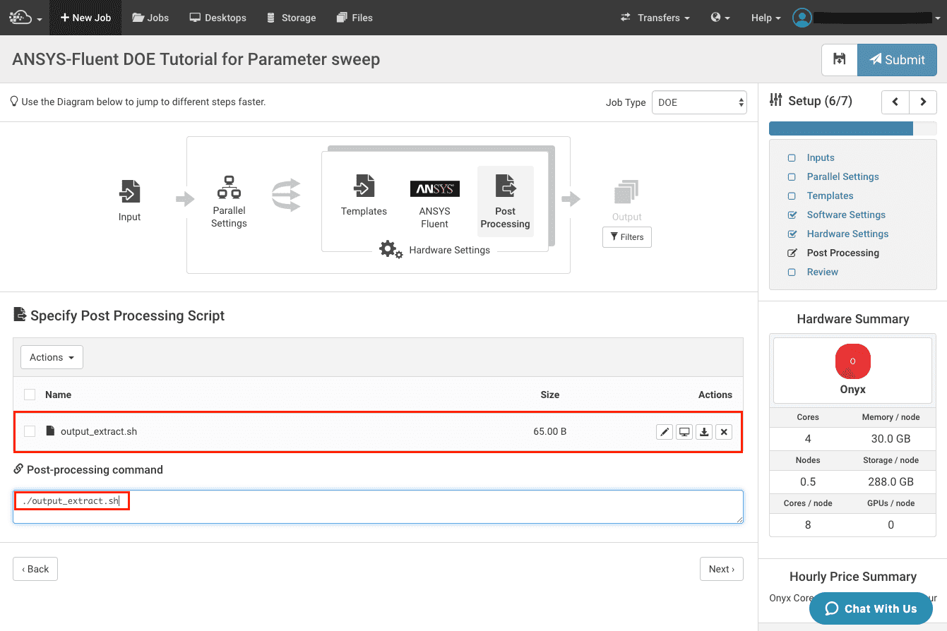
Next, in the Post-processing Command window enter the command to execute the post-processing script as follows:.
bash ./output_extract.sh
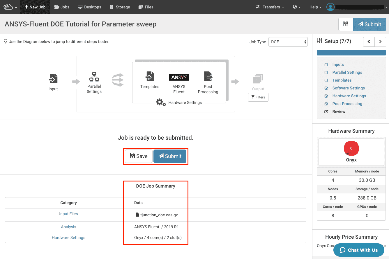
By clicking Next, we can Review the Job setup.
In this section, you can review the job setup:
- DOE Job Summary will list out the input files, software and the hardware settings you have chosen for your analysis.
- The Save and Submit allow you to either save the job setup or submit the job to clusterA computing cluster consists of a set of loosely or tightly ... More.
Once submitted, you will be redirected to the Status page or you can navigate to this page using the Status button on the side panel. When running a DOE Job Type, the Status page will allow users to monitor their runtime files for multiple cases running concurrently using Rescale’s Live Tailingalso referred to as real-time log monitoring or live log str... More feature. In this case, since Task Slots equals 2, two child runs are active at a time, that are indicated by the red box highlighted on the left which shows Runs. The Job Logs indicate the status of each child run.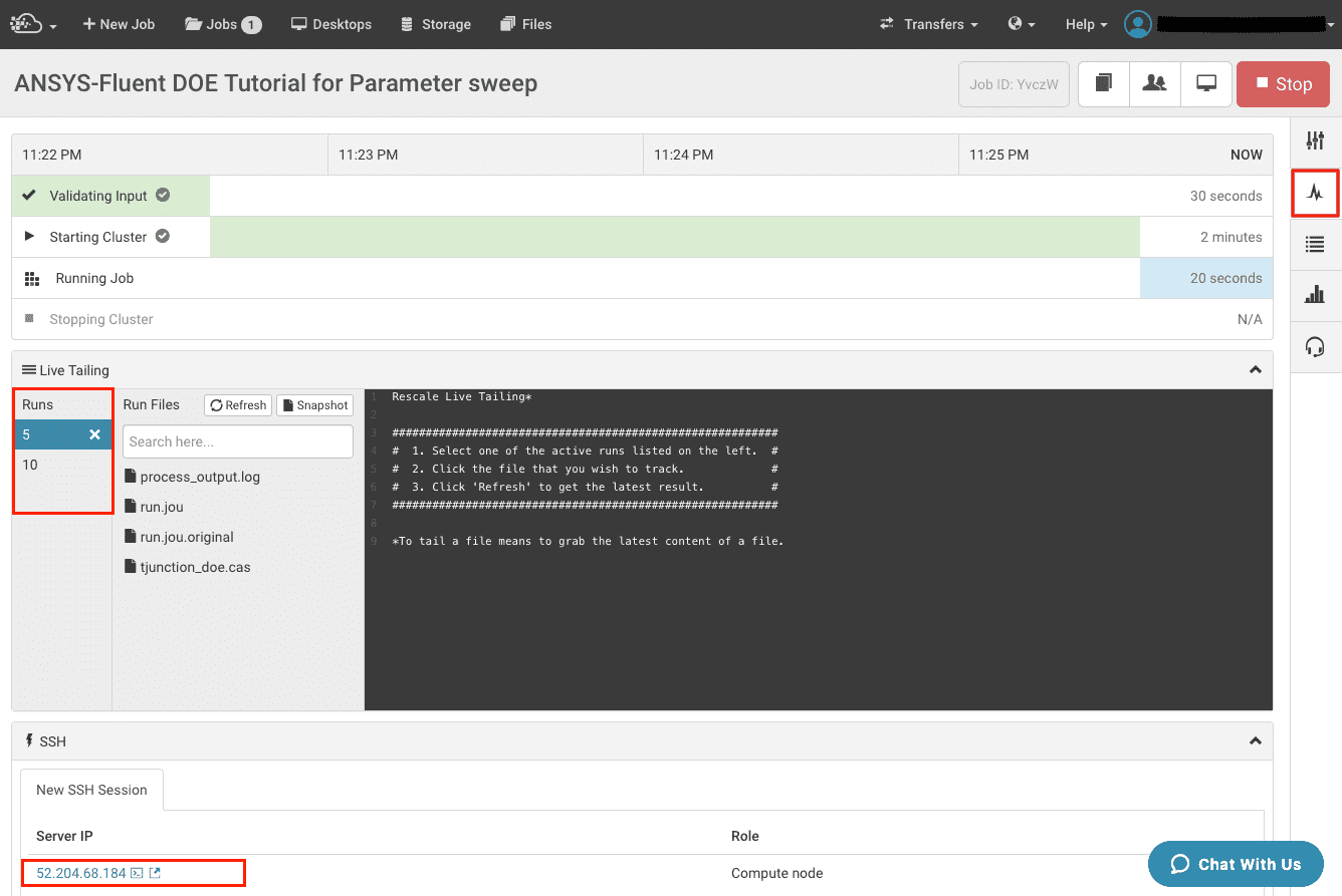
You can also launch an SSH terminal to track you jobs by clicking the IP address link highlighted in red.
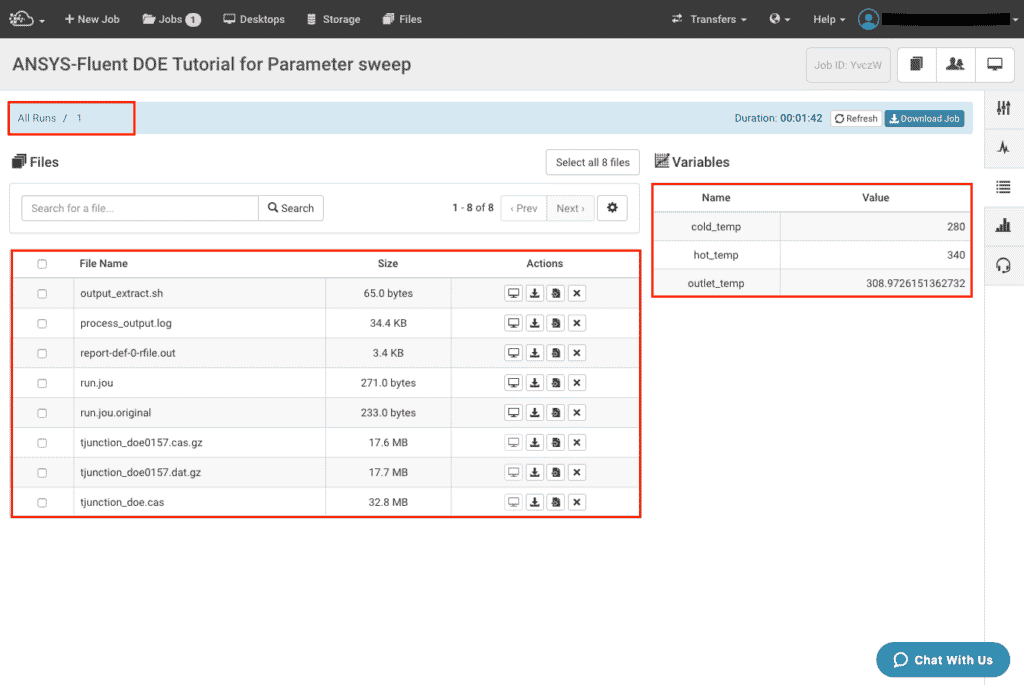
Once the simulations are complete, in the Results page the results of all the runs can be viewed.
The Results page allows you to examine the duration of each run defined in the job, download a zip archive consisting of run files for every case (when complete), download a zip archive consisting of run files for an individual case, or inspect an individual run more closely.
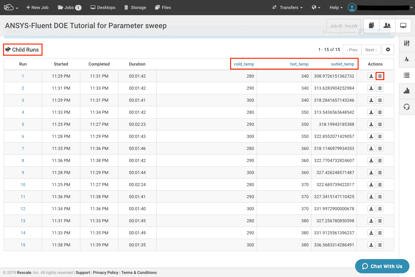
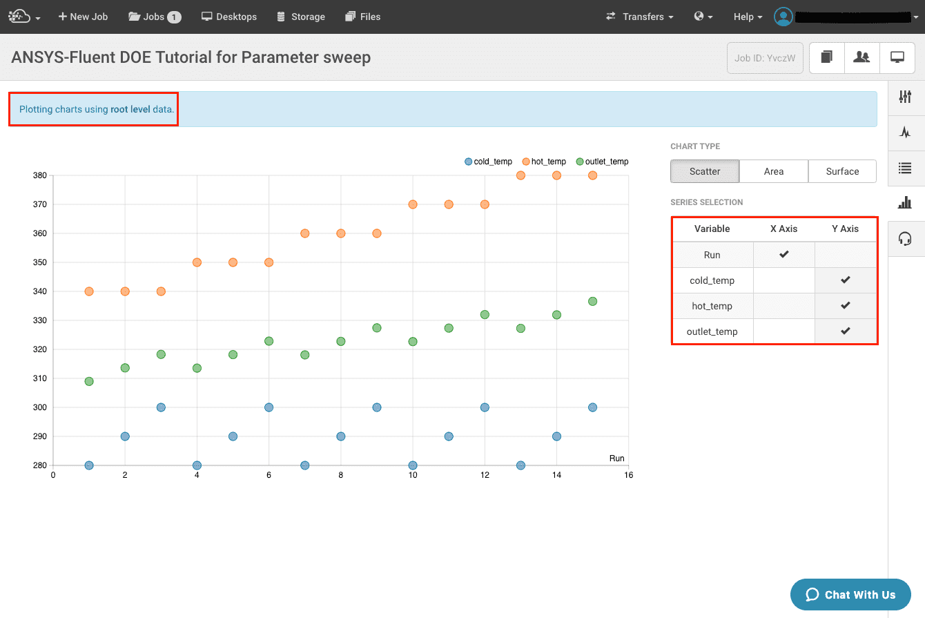
You can access individual runs by clicking the button under actions column highlighted in red. In this page you can see the variables defined on root level and access results obtained from each simulation as seen below:
In the Plotting section you can plot the root level data as shown below: